Random Processes (2)

Random Processes (2)

현재 정리하는 내용은 KAIST EE의 이융 교수님, Probability and Intorductory Random Process 강의를 참고하여 작성했습니다.

Poisson Processes : Poisson RV and Basic Idea

뿌아송~

• 오늘 배울 것은 Poisson process로 BP에서 Continous한 상황을 생각한 방식이다.

Background : Poisson rv X with parameter λ (1)

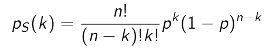
• 예전에 배웠던 Binomial RV에 대해 생각해보면 이 놈의 정의는 다음과 같다.
  → n번의 독립적인 시도에서 성공확률 p를 가질 때, 성공 개수
  → Models the number of successes in a given number n of independent trials with success probability p.

• 공식은 다음과 같다.
  

• 여기서 우리는 궁금해진 것이 있다.
  → 매우매우 큰 n과 매우 작은 p를 가지고 np = λ로 정했을 때, 어떤 일이 발생할까?
  → 즉, np = λ를 가정하고 n이 무한대로 갈 때 어떻게 될까?

  • 여기서 np = λ는 쉽게 생각하면 된다.
    1. n = 1일 때, p = λ
    2. n = 2일 때, p = λ/2
    3. n = n일 때, p = λ/n

• 앞서 나온 공식을 np = λ를 적용해서 lim하기 쉽게 풀게 되면
  
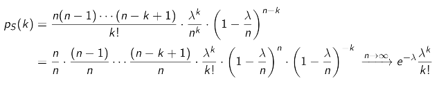
  → 요놈이 Poisson rv이다.
  

  
  

Background : Poisson rv X with parameter λ (2)

• 앞서 찾아낸 Poisson rv의 공식은 다음과 같다.
  

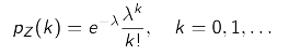
  1. 기본적으로 Binomail을 표방했기 때문에, λ는 nonnegative integer value를 갖는다.
  2. Infinitely many slots(n) with the infinitely small slot duration

• Poisson rv의 Expectation과 var은 다음과 같다.
  
  

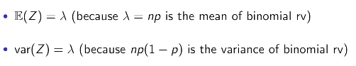
  → 여기서 Expectation은 mean # of arrivals이다.
  → var을 구할 때, np(1-p)에서 n이 무한대로 갈 때를 생각하며 된다.
  
  

Example : Poisson Approximation

• Limit을 취하기 때문에 Approximation이라고 하기도 한다.

• 요놈자식이 어디에 쓰이는지 하나의 예제를 살펴보자.

  A packet consisting of a string of n symbols is transmitted over a noisy channel.

  Each symbol has errorneous transmission with prob. of 0.0001, independent of other symbols.

  Incorrect transmission is when at least one symbol is in error.

  
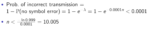
  Question. How small should n be in order for the prob. of incorrect transmission to be less than 0.001?

• 에러 확률은 아주 낮다. 그리고 패킷의 길이가 꽤나 크다.
  → Poisson approximation을 사용하자!

• 간단하다.
  

  

Design of Continuous Analogue of Bernoulli Process

• Remind
  • Geometric vs. Exponential
  • Two rvs with memoryless property
  • conitnuous system is discrete system with infinitely many slots whose duration is infinitely small.
• Independence between what happens in a different time region.
• Memoryless and fresh-start property
• Key Idea : Making it as a limit of a sequence of Bernoulli processes.

Key design idea to develop a Continuous Twin (1)

• Continuous twin

  • Key point : Understand the number of arrivals over a given interval [0, 𝛕]

  • Assume that it has some arrival rate λ.
    

    → Bern Process에서 하나의 슬롯에서의 성공확률 p를 모방한 것
    → # of arrivals / unit time

  • 우리는 discrete time slots의 BP를 다룰 줄 안다.

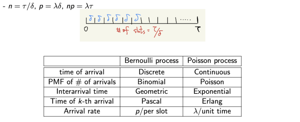
• Limit을 해준다고 했으니 일단은 [0, 𝛕] 구간을 δ의 길이를 갖도록 쪼개주자.
  → Then, n = # of slots = 𝛕 / δ

• 그럼, 여기서 δ를 무한대로 보내버리면 continuous 상황을 만들 수 있을 것이다!

Key design idea to develop a Continuous Twin (2)

• 우리가 갖고 있는 아이디어는 : during one time slot of length δ
• 그럼 모델링을 위해 여기서 3가지의 상황을 생각해보자.
  1. 슬롯에 하나의 도착이 있을 확률
     → arrival rate와 slot length가 관련이 있을 것이다.
     → arrival rate가 높아지면 확률 상승, 반대면 반대 (slog length도 비슷)
  2. 슬롯에 두 개 이상의 도착이 있을 확률
     → 슬롯이 매우 작아지면 거의 없을 법한 확률이다.
  3. 슬롯에 도착이 없을 확률
     → 전체 확률(1)에서 [1]과 [2]의 확률을 빼주면 된다~!
• 수학적으로 이제 생각해보자.
  1. arrival rate와 slot length가 [1]의 확률에 영향을 끼치니
     → λδ
  2. 거의 없을 법한 확률이니까
     → 0
  3. 이건 [1]과 [2]를 빼면 되니까
     → 1 - λδ - 0
• 근데.. 없을 법한 확률이지 완전히 0은 아니다. 따라서 다음과 같이 수정을 해준다.
  1. λδ + o(δ)
  2. 0 + o(δ)
  3. 1 - λδ + o(δ)
• 여기서 o(δ)의 정의는 다음과 같다.
  → Some function that goes to zero faster than delta.
  → Thus, for very small delta, o(δ) becomes negligible, compared to δ.

Key design idea to develop a Continuous Twin (3)

• 지금까지 우리가 생각한 아이디어는 다음과 같다.

  • Given small δ,
    → # of arrivals : ~ Bin(n, p) where n = 𝛕 / δ and p = λδ

  • 그럼 여기서, δ → 0라고 한다면, np = 𝛕 / δ * λδ = λ𝛕
    → Oh! 어디서 봤던 것이다! 바로 Poisson rv!
    

    → [ δ → 0 ] == [ n → INF ]

  • 따라서, 다음이 성립되게 된다.
    
    

    → Expectation = λ𝛕 : mean # of arrivals * time

Poisson Processes: Definition and Properties

Poisson Process: Definition

• An arrival process is called a Poisson process with rate λ, if the following are satisfied :
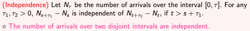
  1. Independence : 두 개의 겹치지 않는 시간대의 # of arrivals는 독립적이다.
     
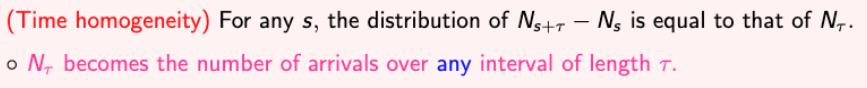
  2. Time homogeneity : 동일한 길이를 갖는 시간대의 # of arrivals의 확률은 동일하다.
     
  3. Small interval probability :
     
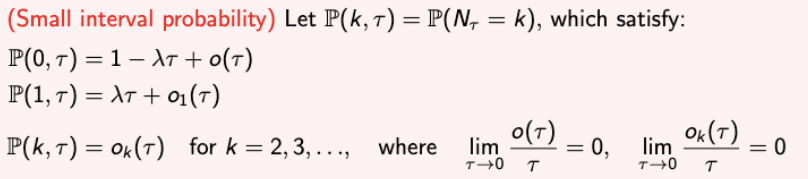
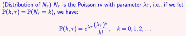
     → 함수 oi(𝛕)는 negligible하다.
  4. Distribution of N𝛕 : (3)의 확장판이다.
     

Poisson Process : P(k, 𝛕), N𝛕 and T

• 이해를 돕기 위해 몇가지 질문을 던져보자.

1. Number of arrivals of any interval with length 𝛕 ~ Poisson(λ𝛕)
   → PP는 ’시간의 위치’가 아닌, ’시간 자체’와 상관이 있다.
   →
   → 따라서, 모든 값에 대해 Poisson RV 값을 갖게 되고.
   

   → 여기서 λ𝛕는 mean # of arrivals를 의미한다. 죽, 0 ~ 𝛕 까지의 시간 중에서의 mean # of arrivals.
   

2. Time of first arrival T
   → Continuous 한 상황에서 생각을 해보자. CDF!
   →
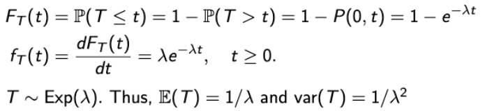
   → 이는 Exp rv임을 알 수 있고, 따라서 memoryless 속성을 갖는다.
   

Poisson Process: Example

• Receive emails according to a Poisson process at rate λ = 5 messages/hour.

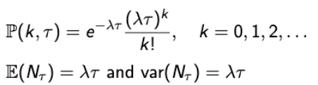
  1. Mean and variance of mails recieved during a day
     → day = 24 hours.
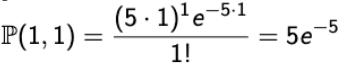
     → E(N𝛕) = var(N𝛕) = λ𝛕 = 5 * 24 = 120
  2. P[one new message in the next one hour]
     → 𝛕 = 1
     →
  3. P[exactly two msgs during each of the next 3 hours]
     → ‘시간의 위치’가 아닌, ‘시간 자체’와 상관 있으며, 따라서 두 개의 겹치지 않는 시간대의 확률은 독립적!
     → P(2, 1) * P(2, 1) * P(2, 1)
     →
     

  
  

  Memoryless and Fresh-start property

  • 이전에 배웠던 Bern. process의 속성과 아주 비슷하지만, 연속적인 시간을 다루기 때문에 time slots이 없음을 먼저 숙지하자.
  • Fresh start. : Start wathcing at time t, then you see the Poisson process, independent of What has happend in the past.
  • Bern. Process에서도 배웠던 k-th arrival time, Yk에 대해서도 생각해보자.
    → k-th interval time을 Tk라고 했을 때, Tk = Yk - Yk-1이 될 것이다.
    
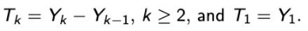
    → 그럼, Yk = T1 + T2 + … + Tk이고 이것은 BP와 달리, sum of i.i.d. exponential RVs이다.
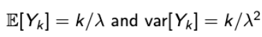
    → T1, T2, …, Tk들은 모두 독립이기 때문에, Exp.과 Var.는 다음과 같이 표현된다. (Linear transform)
    
    

  
  

  PDF of Yk

  • 아주 작은 값 δ가 주어졌을 때,
    → PDF of Yk =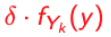 = prob. of k-th arrival over [y, y+δ]
    → 적분을 위해 직사각형을 만든다고 생각하면 된당.
  • 여기서, δ는 아주아주아주 작은 값이기 때문에, 오직 하나의 arrival만 생긴다고 하면 앞의 식은 다음과 같이 전개된다.
    
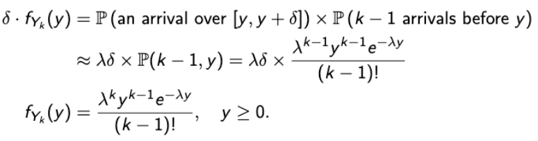
    → 이것을 Erlang rv라고 한다.
  • Erlang rv.
    
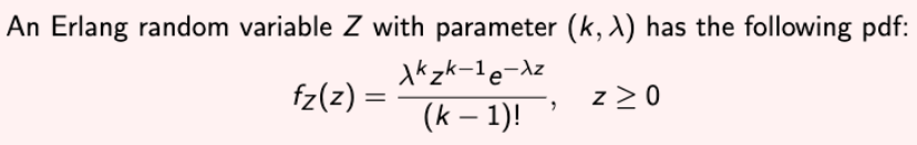
    → Bern. 에서 했던 것과 같이, Erlang(1, λ) = EXP(λ)이다.
    → Bern.에서는 Geom!
    

  
  

  Poisson vs. Bern.

  
  

  
  

  Example: Poisson Fishing

  Catching fish : Poisson process λ = 0.6/hour.

  2시간 동안 낚시를 하게 된다.

  여기서, 2시간 안에 적어도 한 마리의 물고기를 낚는다면, 2시간째에 낚시를 멈춘다(그 동안 몇마리를 잡든 상관 없다.).

  그렇지 않다면 한 마리의 물고기를 낚을 때까지 계속한다.

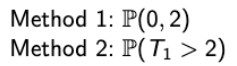
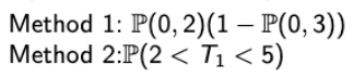
  1. fishing time > 2 hours.
     → 2시간 초과를 한다는 것은, 2시간 동안 한 마리도 못잡았다는 뜻이다.
     

  2. 2 < fishing time < 5
     → 2시간 동안 한 마리도 못 잡았고, 3시간 동안 적어도 한 마리를 낚을 경우이다.
     → 여기서 2시간~5시간이 아닌 3시간이라는 것은 fresh-start 속성 때문이다.
     

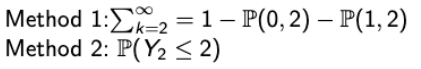
  3. Catch at least two fish
     → 이 때는 적어도 2마리의 물고기를 2시간 이내에 잡아야 할 때이다.
     

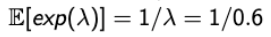
  4. E [ future fishing time | already fished for 3h ]
     → Fresh-start
     → 즉, 3시간 동안 낚은 것은 까먹어버리고 새롭게 한 마리를 잡는 것에 대한 Expectation을 구하면 된다.
     

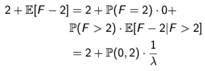
  5. E[ total fishing time ]
     → Expectation은 mean # of arrivals이다. 따라서, 걸린 시간을 다 더해주자.
     

     → 그러면 2시간 전에 걸린 시간(이건 무조건 2시간)과 딱 2시간째, 2시간 이후를 구하면 된다.
     → Continuous에서는 특정 값에 대한 확률은 0이라는 것을 다시 생각하자.
     

  6. E[ number of fish ]
     → 앞의 것과 같지만, λ * 시간 = 물고기 개수!라는 것을 생각해보면 (5)에 λ를 곱해주면 된다.