Random Variables (8)

Radnom Variable (8)

현재 정리하는 내용은 KAIST EE의 이융 교수님, Probability and Intorductory Random Process 강의를 참고하여 작성했습니다.

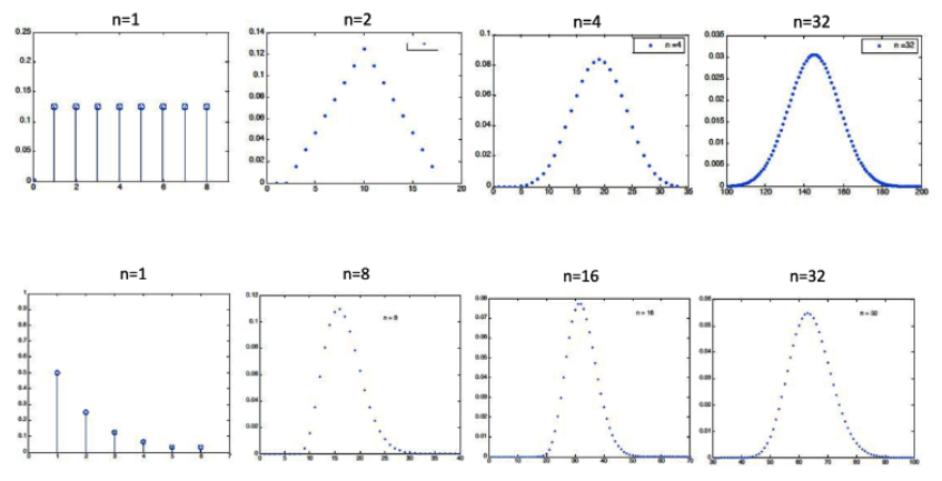
Weak Law of Large Number : Result and Meaning

• 확률 및 랜덤 변수에서 가장 중요한 발견 중 하나이다.

Our interset : Sum of random variables

• RV들의 합이 어떤 의미를 갖는지 간단한 예제를 살펴보자.
  1. n students who decides their presence, depending on their feeling. Each student is happy or sad at random, and only happy students will show their presence. How many students will show their presence?
  2. I am hearing some sound. Their are n noise sources from outside.
• 여기서, 학생의 감정이나 소음의 출처를 X1, X2, … Xn 이라 하고, Xi가 i.i.d라고 해보자.
  → i.i.d : independent and identically distributed
• 그러면, Xi의 Expectation은 μ이고 Variance는 σ^2이 될 것이다.
• 우리가 궁금한 것은 이제 “How the Sum of random variables behaves”이다.
  → 나의 생각이지만 ‘평균 회귀’에 관한 내용 같다. (아직은 잘 모르겠음,,다 안들었음 ㅋㅋ)
  
  

What about distribution of Sn?

• Sn의 distribution을 찾는 것은 매우 어려운 일이다.
• 우리는 저번주에 Z=X+Y의 distribution을 찾을 때도 convolution을 사용하면서 꽤나 힘들었다..
  → 이건 두 개인데 무수히 많은 n은 참으로도 힘들 것이다.
• 단, Sn이 sum of normal rvs라면 Sn도 normal이기 때문에 쉬워지긴 한다.
  → 근데 실제로 이런 일은 거의 없다.
• Possible approach : Take a certain scaling with respect to n that corresponds to a new glass, and investigate the system for large n.

Sample Mean

• Consider the sample mean and try to understand how Sn behaves:
  
  
• E(Mn) = μ , Var(Mn) = (σ^2)/n
• 매우 큰 n에 대해서는 var은 0으로 수렴할 것이다(decays).
• 그럼, Mn은 이것의 randomness를 잃어버릴 것이고, μ값을 중심으로 뭉쳐질 것이다!
• 이것을 Law of large numbers (LLN) 이라고 부른다.

Let’s Establish Mathematically

• 근데, n이 무한대로 갔을 때, 과연 Mn을 μ라고 할 수 있을까?
• n이 무한히 커지면서 var이 0이 되고 Mn은 μ를 중심으로 뭉치니까 그럴 것만 같다.
• 여기서 Ordinary convergence를 확인해보고 가자.
• Ordinary Convergence for the sequence of real number : an → L
  
  
• 이걸 보면, 가정했던 내용이 맞는 것만 같다…하지만 Ordinary Convergence는 real number한테 적용되는 것이고,
  → Mn은 From sample space to Real number 를 해주는 Random variable이다.
• 따라서, 새로운 concept of convergence for the sequence of RVs를 만들 필요가 있다.

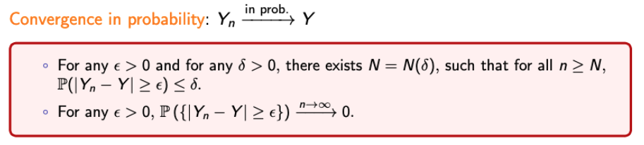
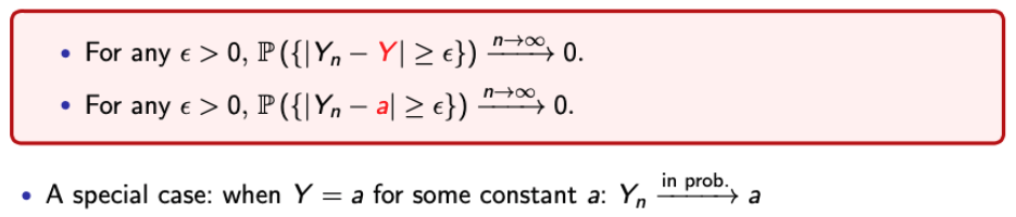
Convergence in Probability (1)

• 아까 말한 것처럼, Ordinary convergence는 real number만 취급해서 우리가 원하는 문제에 적용할 수 없었다…

• 이걸 이용해서 New concept of convergence for the sequence of RVs를 뚝딱 해보자.🔨

• 우리가 원한는 것은 a sequence of rvs (Yn) convergence to a rv Y.

• 먼저, Ordinary convergence를 사알짝 바꿔서 적용해보자.
  
  

  → 이렇게 되면, an은 real number이다. 왜냐면 An이라는 RV이가 sample space에서 real number로 바꿔준 값이 an이기 때문이다.

• 그럼 또 Ordinary convergence를 사알짝 적용해보자.
  
  

  → 짜잔. real number니까 Ordinary convergence가 그대로 적용된다. 물론 ε과 δ의 쓰임 위치를 주의하자.
  

Convergence in Probability (2)

• 그럼,,, Y가 상수가 되면 어떻게 될까?
  → RV의 여러 형태 중 상수가 있으니까!

• 

• 나의 발 그림으로 표현을 해보겠다.
  

  
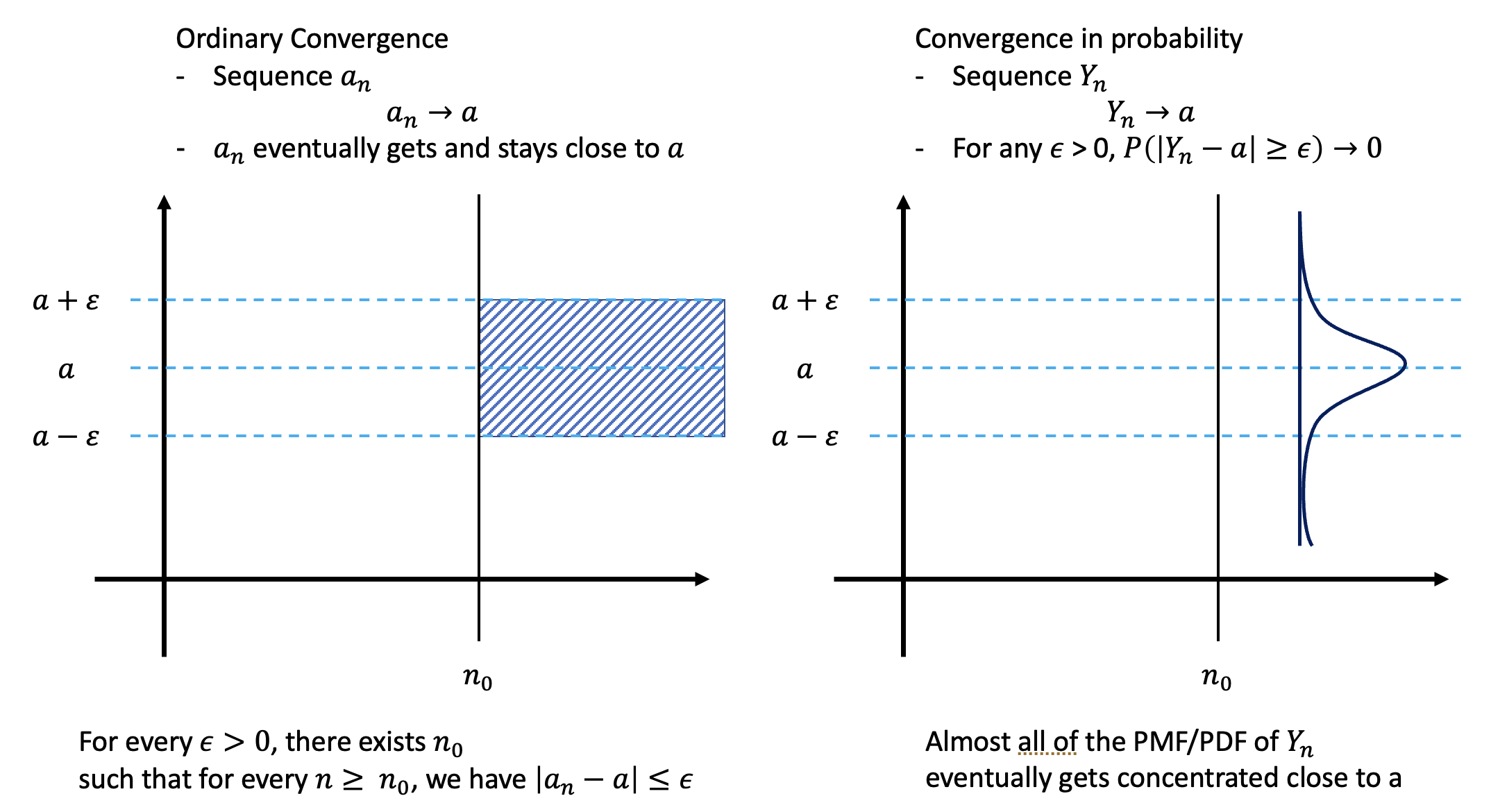
  → 그럼, ε이 작으면 작을 수록 a쪽에 분포할 확률도 높아짐을 알 수 있다.

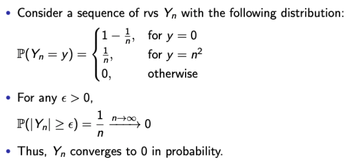
Examples : Convergence in Probability

Exapmle 1.

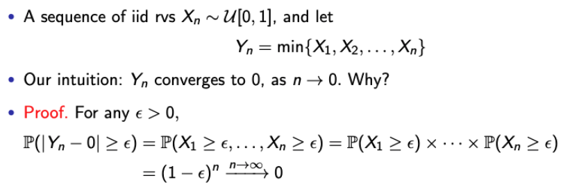
• 최솟값으로 mapping하기 때문에 Y1 >= Y2 >= Y3 >= … >= Yn이다.
• 그럼 무한히 반복되면 당연히 Yn은 0(a)이 수렴할 것이다. → Our intuition

Example 2.

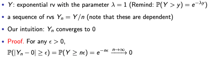
• Y값을 일단 신경쓰지 않아도, n이 커지면 당연히 Yn은 0에 수렴할 것이다.

Example 3.

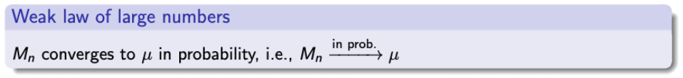
Weak Law of Large Number (WLLN)

• 우리가 지금까지 사용했던 Mn은 간단하게 말하자면, μ 주변으로 값이 모인다라는 것이다.
  

WLLN : Why useful?

1. If we take the scaling of Sn by 1/n, it behabes like a deterministic number. This significantly simplfies how we understand the world.
   

   → For example, assume that a large number of identically distributed noise come to you. Then, you can roughly approximate it as n*average noise.

2. Provides an interpretation of expectation in terms of a long sequence of identical independent experiments.
   → For example, what is the probability of head of a coin?
   → Toss 1000 times, and count the number of heads.

Central Limit Theorem : Result and Meaning

Central Limit Theorem : Start with Scaling (1)

• 이전에 배웠던 WLLG를 loosely하게 얘기하면
  
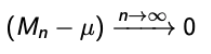
• 그러나 우리는 어떻게 (Mn-μ)가 0으로 수렴되는지는 알지 못한다.
• Question. What should be “somthing”?
  
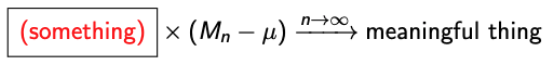
  → (Mn-μ)은 0으로 수렴하니까, Something should blow up for large n.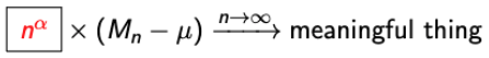
  
  
• 그럼 여기서 α는 몇이 되어야 할까?
  → 1/2 (왜?????왜?????????? 모르겠다!!!!!!!!!)

Central Limit Theorem : Start with Scaling (2)

• 나의 궁금증이 이제야 풀리는도다.
• 먼저, 앞서 작성한 식을 reshape해보자.
  
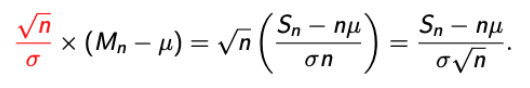
  → 시그마를 붙인 이유는 식의 아름다움을 위함이다. 뒤에 가면 느껴진다.
• 자, 여기서 나온 식을 Zn이라고 해보자.
  
  → 이렇게 되면, Zn is well-centered with a variance irrespective of n.
• 우리는 이를 통해 Zn이 n이 무한대로 갈 때, 어떤 의미있는 무언가로 수렴하게 만들었다. 무언가가 무엇일까??
  → Interestingly, it converges to some well-known random variable. (Zn → Z)
  → 이제 이게 어떤 놈으로 나올지 알기 위해, Need a new concept of convergence : Convergence in distribution

Convergence in Distribution

• 이전과 같이 a sequence of res (Yn) and a rv Y 를 생각해보자.
• 
  → Another type of convergence of RVs
  → Convergence in probability → Convergence in distribution, but the reverse is not true.
• 증명은 나중에 하도록 하고, 이해하기 위한 예제를 보고 가자.

Example : in Distribution but not in Probability

• 1 이상의 정수 n에서, 베르누이 RV Xn이 있다고 해보자.
• 그리고 X = 1 - Xn이라고 해보자.
  → Xn은 누가 되었든 Bern(1/2)일 것이고, 따라서 X ~ Bern(1/2)이다.
  → 그렇다는 것은 distribution of Xn and distribution X are equal.
  → This is trivial that Xn converges to X in distribution.
• 그럼 Convergence in probability는???
  
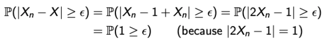
  → 역이 성립 안된다고 했으니 그렇다.

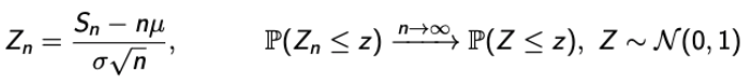
Central Limit Theorem : Formalism

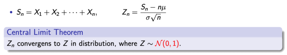
• 아까 누구로 변하는지 확인한다고 했다!
• 바로바로 CLT를 통해 Standard Normal Random Variable로 변환이 된다.
  → Irrespective of the distribution of Xi, Z is normal.

LLG vs CLT : Different Scaling Glasses

• 둘 다 ‘안👓경’을 끼고 새로운 세계로 가는 방식이다.
• 안경을 낀 순간 두개가 어떤 세계로 가는지 확인해보자.

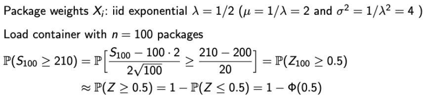
Practival Use of CLT

• 지금까지 배웠던 CLT를 식으로 표현하면 다음과 같다.
  
  → Zn을 Standard Normal RV로 근사시키는 역할을 한다.
• 그럼 여기서 Zn에 대한 식이 아닌 Sn에 대한 식으로 변환하면, 이 또한 Normal rv가 된다.
  
• 그럼, n이 얼마나 커야할까…?
  1. 보통은 20~30정도가 적당하다.
  2. Distribution of Xi가 symmetry or unimodality라면 더 작은 n도 작동한다.
     → Unimodality : A single maximum or minimum. 낙타 봉같은 모습이 아닌 종 모양이라고 생각하면 됨.

CLT : Examples of Required n

Examples

Examples of CLT (1)

• n과 a가 주어졌을 때, b를 구해보자.
  

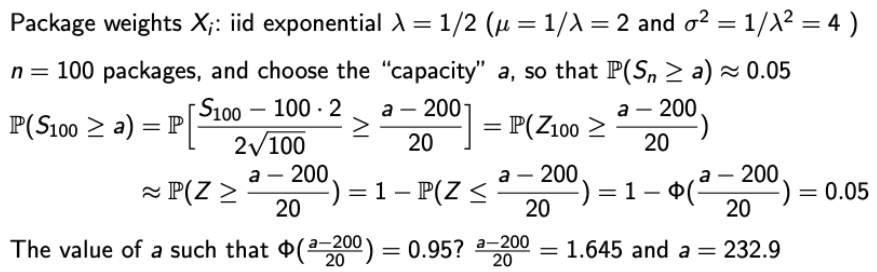
Examples of CLT (2)

• n과 b가 주어졌을 때, a를 구해보자.
  
  

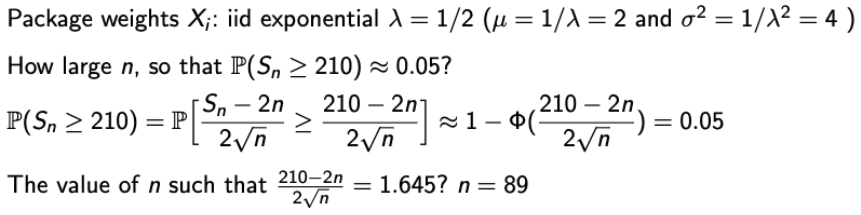
Examples of CLT (3)

• a와 b가 주어졌을 때, n을 구해보자.